Note
22/3/2023: Revised.
6/2/2021: Table of Formulae last two columns merged.
11/3/2020: Interest rate "may be" changed to "must be" when converting to monthly interest rate.
10/3/2020: Conversion from annual interest rate to monthly interest rate added.
28/1/2019: Revised to re-arrange the order and give a simpler summary of the formulae.
7/2/2018: Created.
Time Value of Money
Generally
- $1 in possession now can earn interest by saving in a bank.
- $1 borrowed now will incur interest until the $1 is repaid.
- $1 can buy more things now than in the future because the commodity prices generally increase over time due to inflation.
- Therefore, $1 received in the future will be of less value than $1 received now.
- Similarly, $1 paid in the future will be less expensive than $1 paid now.
- When comparing amounts paid over different times, they should be converted to their equivalent values at the same time for comparison on the same basis.
- They may be converted to the present value (present time) or future value (future time) or annuity (annually).
(added, 22/3/2023)
Interest on Loan
- Simple interest = Interest calculated only on the original amount (principal) loaned.
- Compound interest = Interest calculated on the original amount and accumulated interests.
- Total amount to be repaid for $100 principal at interest rate (R%) of 10% per annum:
|
Loan $100 Now |
Repay by End of 1 Year |
Repay by End of 2 Years |
Repay by End of 3 Years |
Repay by End of N Years |
|
Simple interest |
100 + 10 = 110 |
100 + 10 x 2 = 120 |
100 + 10 x 3 = 130 |
Loan x (1 + R% x N) |
|
Compound interest |
100 x (1 + 10%) = 110 |
110 x (1 + 10%) = 121 |
121 x (1 + 10%) = 133 |
Loan x (1 + R%)N |
- Money borrowed now will need repayment in a bigger amount in the future. A longer loan will cost more.
Same Money Paid Later Costs Less Now
- On the other hand, if the same amount of loan can be paid later, the cost of the loan will be less.
- If a buyer needs to borrow money to pay to buy something, and if he can borrow and pay the same price later, the cost of the loan will be less, and therefore later payment will cost less.
- If a buyer does not need to borrow money to pay, and if he can pay the same price later, he can use the spare money now to invest elsewhere to earn money, and therefore later payment will cost less.
(revised, 22/3/2023)
Compounding (PV --> FV)
- Converting the present value to the future value is called compounding, because compound interest rates are usually used.
(revised, 22/3/2023)
Discounting (PV <-- FV)
- Converting the future value to the present value is called discounting, because the present value is less than the future value of the same amount of money to be paid.
(revised, 22/3/2023)
Factors
- Factors are used to simplify all discounting and compounding calculations whereby:
- Result $ = Base $ x Factor per $1
- Future value = Present value x Compounding factor
- Present value = Future value x Discounting factor.
(revised, 22/3/2023)
Definitions
- PV = Present value | present worth | principal amount invested now.
- FV = Future value | future worth | terminal value | terminal worth.
- A = Annuity, a periodic payment.
- N = Number of period (year, quarter, month, week or day).
- R% = % rate of interest | rate of return | discount rate applicable at the end of a period.
- C = 1 + R%.
- Due means payable at the beginning of a period.
(revised, 22/3/2023)
Table of Formulae (compound interest)
|
Factor Description |
Formula |
|---|---|
|
CN |
|
1 / (FV of 1) = 1 / CN |
|
(CN - 1) / R% |
|
1 / (FVA of 1 after N) = R% / (CN - 1) |
|
(CN - 1) * C / R% |
|
1 / (FVA Due of 1 after N) = R% / C / (CN - 1) |
|
(1 - 1 / CN) / R% |
|
1 / (PVA of 1 after N) = R% / (1 - 1 / CN) |
|
(CN - 1) / CN - 1 / R% |
|
1 / (PV of A Due of 1 after N) = R% * CN - 1 / (CN - 1) |
(Verification, after 12 times per year for a year, N = M = 12, (1 + R%) N/M becomes (1 + R%), the FV of $1 after 1 year.) |
Used by banks: Interest rate, X% = R%/M. Compounding factor, FV of $1 after N times = (1 + X%) N = (1 + R%/M) N Discounting factor, PV of $1 after N times = 1 / (1 + X%) N = 1 / (1 + R%/M) N Accurate: Interest rate, X% = (1 + R%)1/M – 1. Compounding factor, FV of $1 after N times = (1 + X%) N = (1 + R%)N/M Discounting factor, PV of $1 after N times = 1 / (1 + X%) N = 1 / (1 + R%) N/M |
Note: X / Y / Z = X / (Y * Z), e.g., 8/4/2 = 1; 8 / (4 * 2) = 1; but the former is easier for manual calculation or setting formulae in Excel, therefore, the former format is used above.
(revised, 22/3/2023)
Examples
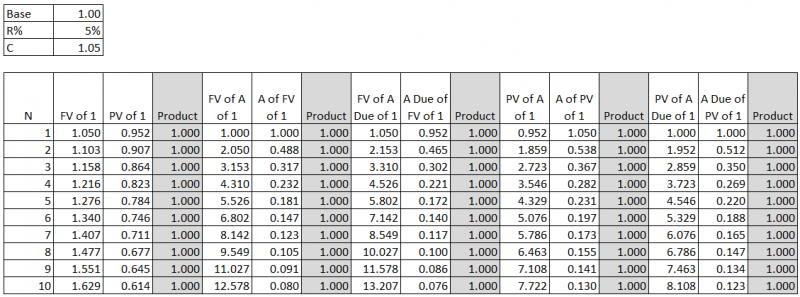
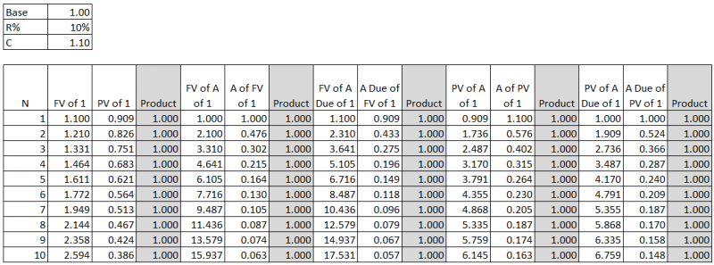
- Note: The above shows that if the interest rate is higher, the future value will be bigger but the present value is smaller.
- Diagrammatically:
- PV --> FV = add 10% to compound PV to FV
- PV <-- FV = divide by 1.1 to discount FV to PV
- [1] = add payment of 1 monetary value.
- FV of [1]:
| [1] --> 1.1 | 1.1 --> 1.21 | 1.21 --> 1.331 |
- PV of [1]:
| 0.751 <-- 0.826 | 0.826 <-- 0.909 | 0.909 <-- [1] |
- FV of A of [1]:
| 0 --- [1] | 1 --> 1.1 + [1] = 2.1 | 2.1--> 2.31 + [1] = 3.31 |
- A of FV of 1 = 1 / (FV of A of 1):
| 1 / 1 = 1 | 1 / 2.1 = 0.476 | 1 / 3.31 = 0.302 |
- FV of A Due of [1]:
| [1] --> 1.1 | 1.1 + [1] = 2.1 --> 2.31 | 2.31 + [1] = 3.31 --> 3.641 |
- A Due of FV of 1 = 1 / (FV of A Due of 1):
| 1 / 1.1 = 0.909 | 1 / 2.31 = 0.433 | 1 / 3.641 = 0.275 |
- PV of A of [1] = FV of A of [1], all discounted back to now by dividing by 1.10 for each period:
| 0.909 <-- 1 | 1.736 <-- 1.909 <-- 2.1 | 2.487 <-- 2.736 <-- 3.009 <-- 3.31 |
- A of PV of 1 = 1 / (PV of A of 1):
| 1 / 0.909 = 1.1 | 1 / 1.736 = 0.576 | 1 / 2.487 = 0.402 |
- PV of A Due of [1] = FV of A Due of [1], all discounted back to now by dividing by 1.10 for each period:
| 1 <-- 1.1 | 1.909 <-- 2.10 <-- 2.31 | 2.736 <-- 3.009 <-- 3.31 <-- 3.641 |
- A Due of PV of 1 = 1 / (PV of A Due of 1):
| 1 / 1 = 1 | 1 / 1.909 = 0.524 | 1 / 2.736 = 0.365 |
(revised, 22/3/2023)
FV of $1 paid now at simple interest (1 payment)
- Also called "Future Value Factor" or "Amount of $1"
- A principal of $1 invested now earning R% interest per number of period
- After 1 period, FV of 1 = 1 + 1 * R% = 1 + R%
- Interest earned taken away leaving the principal there for the next period
- Base to earn interest for the 2nd period, still = 1
- After 2 periods, FV of 1 = 1 + R% + R% = 1 + 2 * R%
- After N periods, FV of 1 = 1 + N * R%
- FV of $1 after N periods
= 1 + N * R% (at simple interest)
FV of $1 paid now at compound interest (1 payment)
- Also called "Future Value Factor" or "Amount of $1"
- A principal of $1 invested now earning R% interest per number of period
- After 1 period, FV of 1 = 1 + 1 * R% = 1 + R%
- Interest earned kept with the principal there for the next period
- New base to earn interest for the 2nd period = 1 + R%
- After 2 periods, FV of 1 = (1 + R%) * (1 + R%)
- After N periods, FV of 1 = (1 + R%)N
- FV of $1 after N periods
= (1 + R%)N (at compound interest)
= CN
PV of $1 paid after N periods at compound interest (1 payment)
- Also called "Present Value Factor"
- PV * (FV of 1) = FV
- PV = FV / (FV of 1)
- PV of 1 in the future = 1 / (FV of 1)
- Since FV of 1 = CN
- PV of $1 after N periods
= 1 / CN
FV of an Annuity of $1 paid at the end of each period after N periods at compound interest (N payments)
- Also called: "Future Value of $1 per annum" if the period is a year
- $1 invested at the END of each of N periods earning R% interest per number of period
- One way to calculate the future sum:
- FV of 1 = CN
- FV of 1 invested 1 period later for N-1 periods = CN-1
- FV of 1 invested 2 periods later for N-2 periods = CN-2
- FV of 1 invested N-1 periods later for 1 period = C
- FV of 1 invested N periods later for 0 period = 1 (no interest)
- Sum = CN-1 + CN-2 + .... + C2 + C + 1
- Another way to calculate the future sum:
- Sum after 1 period with 1 invested at the end = 1
- with sum earning interest next period and another 1 invested at the end of next period
- Sum after 2 periods = C + 1
- Sum after 3 periods = C2 + C + 1
- Sum after N-1 periods = CN-2 + ... + C2 + C + 1
- Sum after N periods = CN-1 + CN-2 + ... + C2 + C + 1
- Sum = CN-1 + CN-2 + .... + C2 + C + 1
- Mutiply all on both sides by C
- Sum * C = CN + CN-1 + CN-2 + .... + C2 + C
- Subtract between the two equations
- Sum * R% = CN - 1
- Sum = (CN - 1) / R%
- Therefore
- FV of A of $1 after N periods
= (CN - 1) / R%
Annuity (e.g. sinking fund) paid at the end of each of N periods to give FV of $1 at compound interest (N payments)
- Find A where (FV of A after N) = 1
- FV of A after N = A * (FV of A of 1 after N) = 1
- A after N periods to give FV of $1
= 1 / (FV of A of 1 after N)
= R% / (CN - 1)
FV of an Annuity Due of $1 paid at the beginning of each period after N periods at compound interest (N payments)
- $1 invested at the BEGINNING of each of N periods earning R% interest per number of period.
- This is equivalent to keeping the total money at the end and investing it for 1 more period to earn interest without adding 1 at the end of the 1 more period:
- FV of A Due of $1 after N periods
= (FV of A of 1 after N) * C
= (CN - 1) * C / R%
- Compare with (FV of A of 1 after N+1) - 1
= (CN+1 - 1) / R% - 1
= (CN+1 - 1 - R%) / R%
= [CN+1 - (1 + R%)] / R%
= (CN+1 - C) / R%
= (CN - 1) * C / R%
- Therefore, FV of A Due of 1 after N
also = (FV of A of 1 after N+1) - 1
diagrammatically:
0-----1 = payment of 1 at the end of a period
-->-- = a period with interest
0-----1-->--1-->--1 = FV of A of 1 after N payments, compounding for N-1 periods
0-----1-->--1-->--1-->--1 = FV of A of 1 after N+1 payments, compounding for N periods
1-->--1-->--1-->--0 = Subtract 1 at the end = FV of A Due of 1 after N payments, compounding for N periods
Annuity Due (e.g. sinking fund) paid at the beginning of each period after N periods to give FV of $1 at compound interest (N payments)
- Find A where (FV of A Due after N) = 1
- FV of A Due after N = A * (FV of A Due of 1 after N) = 1
- A Due after N periods to give FV of $1
= 1 / (FV of A Due of 1 after N)
= R% / [(CN - 1) * C]
= R% / (CN - 1) / C
PV of an Annuity of $1 paid at the end of each period after N periods at compound interest (N payments)
- Also called: "Present Value of $1 per annum" or "Years Purchase" if the period is a year
- $1 paid at the END of each of N periods to be discounted back to the present value at R% interest per number of period passed
- Instead of discounting the individual payments back for different periods, the total future value of all payments after N is discounted back once
- PV of A of $1 after N periods
= (FV of A of 1 after N) * (PV of 1 after N)
= [(CN - 1) / R%] * (1 / CN)
= (CN - 1) / CN / R%
= (1 - 1 / CN) / R%
= (1 / CN - 1) / R% * (-1), for easier manual calculation
= [1 - (PV of 1 after N)] / R%
Annuity paid at the end of each period after N periods to equal $1 now at compound interest
- Find A where (PV of A after N) = 1
- PV of A after N = A * (PV of A of 1 after N) = 1
- A after N periods to equal $1 now
= 1 / (PV of A of 1 after N)
= R% * CN / (CN - 1)
= R% * [1 + (CN - 1)] / (CN - 1)
= [R% + R% * (CN - 1)] / (CN - 1)
= R% / (CN - 1) + R%
= (A after N to give FV of 1) + R%
which can be considered as of two portions
= Sinking fund at end of each period to repay the loan at the end + interim loan interest R%, where the R% for the sinking fund may be different from the R% for loan interest.
PV of an Annuity Due of $1 paid at the beginning of each period after N payments at compound interest (N - 1 periods)
- $1 paid at the BEGINNING of each of N periods to be discounted back to the present value at R% interest per number of period passed
- Instead of discounting the individual payments back for different periods, the total future value of all payments after N is discounted back once
- PV of A Due of $1 after N periodic payments
= (FV of A Due of 1 after N) * PV of 1 after N periodic payments
= [(CN - 1) * C / R%] * (1 / CN)
= (CN - 1) * C / CN / R%
= C * (CN - 1) / CN / R%
= C * (PV of A of 1 after N periodic payments)
= (CN - 1) / CN-1 / R%
- This is equivalent to discounting by 1 less period as compared with paying the annuity at the end of each period.
- The discounting factor for 1 more period = * 1 / C
- The discounting factor for 1 less period = * C
- Compare with (PV of A of 1 after N-1) + 1, which is
= (CN-1 - 1) / (R% * CN-1) + 1
= (CN-1 - 1 + R% * CN-1) / (R% * CN-1)
= (CN-1 * (1 + R%) - 1 ) / (R% * CN-1)
= (CN-1 * C- 1 ) / (R% * CN-1)
= (CN - 1 ) / (R% * CN-1)
= C * (CN - 1) / (R% * CN)
Therefore, PV of A Due of 1 after N
also = (PV of A of 1 after N-1) + 1
diagrammatically:
--<-- = Discounting with interest
0--<--1--<--1--<--1--<--1 = PV of A of 1 after N payments, discounting for N periods
0--<--1--<--1--<--1 = PV of A of 1 after N-1 payments, discounting for N-1 periods
1--<--1--<--1--<--1 = Add 1 to the beginning = PV of A Due of 1 after N payments, discounting for N-1 periods
Annuity Due paid at the beginning of each period after N payments to equal $1 now at compound interest (N - 1 periods)
- Find A Due where (PV of A Due after N) = 1
- PV of A Due after N = A * (PV of A Due 1 after N) = 1
- A Due after N payments to give $1 now
= 1 / (PV of A Due of 1 after N)
= 1 / [(CN - 1) / CN-1 / R%]
= R% * CN-1 / (CN - 1)
Converting Nominal Annual Compound Interest Rate to Compound Interest Rate for M Times Regular Payments in a Year for N Times
- From the above, FV of 1 after N @ R% interest rate each time = (1 + R%)N.
- When N = years, R% = annual interest rate.
- When N = times, R% = interest rate each time. Let’s call it X%.
- When there are M times regular payments in a year, the usual method used by banks to calculate the interest rate X% each time is:
- X% = R% / M
- Accurate method:
- Compounding at X% interest rate each time after M times a year for 1 year should be equal to (1 + R%)
- (1 + X%)M = (1 + R%)
- (1 + X%) = (1 + R%) 1/M
- X% = (1 + R%) 1/M – 1
- Test based on R = 10%, M = 12 for 1 year:
- Banks’ method:
- monthly rate = 10%/12 = 0.000833
- compounded total after 1 year = (1 + 10%/12)12 = 1.1047
- Accurate method:
- monthly rate = (1 + 10%)1/12 – 1 = 0.007974
- compounded total = (1 + 0.007974)12 = 1.10
- Compare with annual compounding only:
- (1 + 10%) = 1.10
- Banks’ method:
- FV of 1 after compounding at M times a year for N times at X% discount rate each time
- = (1 + X%) N
- = [1 + (1 + R%) 1/M – 1] N
- = [(1 + R%) 1/M] N
- = (1 + R%) N/M
- An easier way to remember:
- Let F be the compounding factor each time
- F compounded for M times a year should be equal to (1 + R% annual interest rate)
- F M = (1 + R%)
- F = (1 + R%) 1/M
- F compounded for N times should become:
- F N = (1 + R%) N/M
- PV of 1 after compounding at M times a year for N times at X% discount rate each time
- = 1 / FV
- = 1 / (1 + X%) N
- = 1 / (1 + R%) N/M
(revised, 22/3/2023)
Inflation, Deflation and Escalation
- Inflation is a general increase in the prices of goods and services in an economy over a period of time.
- Deflation is a general decrease in the prices of goods and services in an economy over a period of time.
- Escalation is a general increase in the prices of specific group of goods and services over a period of time.
- For simplicity, an inflation rate or escalation rate may be positive or negative.
- When the inflation rate or escalation rate (E%) is said to be 10% per annum year on year. It means that the price in a year is 10% high than the price a year ago, e.g.:
|
Now |
End of 1 Year |
End of 2 Years |
End of 3 Years |
|
Present price = 100 |
100 x 1.1 = 110 |
100 x 1.1 x 1.1 = 121 |
100 x 1.1 x 1.1 x 1.1 = 133 |
- The purchasing power of the same amount of money decreases with inflation. Alternatively, it is said to have a devaluation of the money.
- One has to cumulate more money to buy the same quantity of goods and services (assuming same quality and still available) in the future.
- The future cost to buy = current cost x (1 + E%)N.
- In principle, discounting to the present value should be based on:
- discounted cost = future cost x discounting factor.
- The future cost should be the cost taking into account the impact of inflation and escalation, and is called “nominal cost”.
- The future cost can only be estimated based on:
- future cost = current cost x escalation factor, where the escalation (specific) is inclusive of inflation (general).
- Therefore, discounted cost = current cost x escalation factor x discounting factor.
- General inflation is difficult to predict. Since it lowers purchasing power, the discount rate used to calculate the discounting factor has to compensate the decrease in purchasing power. The discount rate is called “nominal discount rate”. Since both the inflation factor and the adjustment to the discount rate apply to all goods and services being considered for comparison, it is considered in order to ignore the general inflation and the corresponding adjustment to the discount rates.
- The cost exclusive of the impact of general inflation is called “real cost”. The corresponding discount rate excluding the impact of general inflation is called “real discount rate”.
- However, for a specific group of goods and services, their escalation rates can be different from the general inflation rates, it is suggested by some people that their future costs should be based on the differential escalation rates beyond the general inflation rates, while the real discount rates are still used.
- Therefore, the above equation can be re-written as:
- discounted cost = nominal cost x nominal discounting factor
- discounted cost = real cost x escalation factor x nominal discounting factor
- discounted cost = real cost x real discounting factor
- discounted cost = current cost x differential escalation factor beyond general inflation factor x real discounting factor
- discounted cost = current cost x (1 + E%)N / (1 + R%)N,
- where E% is the full or differential escalation rate
- R% is the nominal discount rate or real discount rate respectively.
- The above shows that:
- escalation factor x nominal discounting factor = real discounting factor
- (1 + E%)N / (1 + nominal R%)N = 1 / (1 + real R%)N
- (1 + E%) / (1 + nominal R%) = 1 / (1 + real R%)
- (1 + nominal R%) = (1 + E%) * (1 + real R%)
- nominal R% = (1 + E%) * (1 + real R%) - 1
- nominal R% = E% + real R% + E% * real R%, the last product is very small and can be ignored
- i.e., nominal discount rate = escalation rate + real discount rate
- or, real discount rate = nominal discount rate – escalation rate
- ISO 15686-5 suggests to use real costs and real discount rates, and assume no differential escalation rates first, but then adjust the discount rates while doing sensitivity analysis to test the impact of the possible differential escalation rates.
(added, 22/3/2023)
Guidance on Discount Rates given by ISO 15686-5 (cited in italics)
- The type of discount rate, either real or nominal, shall be clearly distinguished.
- NOTE 1 The real discount rate applied to costs (and benefits) that are also measured in real terms assumes that inflation/deflation applies equally to all.
- Occasionally, escalation rates may be used as a form of sensitivity analysis where there are grounds to anticipate that the standard rate of inflation does not apply in the case of a specific scenario. Typically, real rates should be used; these exclude the impact of future inflation. Nominal rates may be used by agreement, if that is what is required by the client or justified by the situation.
- The discount rate in the private sector should represent the opportunity cost of investing the capital, which can be:
- a) the interest cost of a loan for the investment;
- b) the interest lost on reduction of cash on deposit;
- c) the returns lost on investment elsewhere (e.g. in bonds or equities);
- d) the actual return achieved on capital investment in the business;
- e) the required rate of return of an investor in a new business.
- Within the public sector, a discount rate can be determined by the central government (sometimes termed the social discount rate) as a test requirement for their investments, based on an assessment of the long-term opportunity cost to the public sector of selecting one investment rather than another.
- NOTE 2 Historically, the real discount rate has reflected the general productivity rate of the producer, sector or field. Generally, productivity has been within 0 % and 2 % over the long term. However, rates as low as these are not universal. Discount rates of between 0 % and 4 % are typically used. A higher rate discourages long-term investments, while a lower rate encourages them.
- NOTE 3 Where the discount rate is not a requirement fixed by the client (public or private), it is normal to undertake sensitivity analysis using a range of rates to test the validity of the conclusions if the input conditions change.
(added, 22/3/2023)
Tax
- If the discount rates are based on investment interest rates which are subject to tax, the discount rates should subtract the tax charged, e.g., interest rate x (1 – % tax on interest rate).
(added, 22/3/2023)
Sensitivity Analysis
- In life cycle costing, since the discount rates are estimates only, it is suggested that discount rates should be adjusted up or down within the possible range to test whether the relative order of the costs of the options would be changed or not. If not, the choice will be more certain. If changed, more careful review should be taken.
- The same apply to other data which may likely be varied.
(added, 22/3/2023)
Life Cycle Costing 生命周期成本計算
- Mainly for comparing between different options with different expenditure patterns over a long period of years of use.
主要用來比較在很長的使用年期有不同的支出幅度的不同方案。 - Considering the whole life cost of a project (or product, service) from birth to death (or before recycling).
考慮某項目(或產品、服務)由生到滅(或再生前)的全部成本。 - Using discounted cash flow techniques to convert monies spent over different times to the same base.
用貼現金流的方式把不同時間支出的金錢轉換到同一基準上。 - Impacts on the use of natural resources are now also under the scope of consideration.
對自然資源使用的影響現在亦納入考慮範圍。
Life Cycle Costs 生命周期成本
- Scope:
- Initial | Capital Costs
初始 | 資本費用 - Costs-in-use:
使用費用- Routine Operation, Maintenance and Repair Costs
日常的使同、保養及維修費用 - Renewal | Replacement Costs
更新 | 更換費用
- Routine Operation, Maintenance and Repair Costs
- End of Life Costs (Removal and Disposal Costs less Residual | Resale | Salvage Values)
終結費用(清拆及處置費用減剩餘價值(轉售價值或廢品價值)) - Non-Monetary Benefits or Costs.
非金錢的益處或成本
- Initial | Capital Costs
- The total of the above is also called “Total Cost of Ownership”.
- “|” = separator between alternative terms.
(revised, 22/3/2023)
Present Values of Life Cycle Costs
- Being sum of:
- Initial | Capital Costs
- (spend now) * 1
- Costs-in-use
- Routine Operating, Maintenance, and Repair Costs
- (average amounts spent every year) * (Present value of annual payment of $1 after N years)
- Replacement or Renewal Costs
- (specific amounts spent after M years) * (Present value of $1 after M years)
- Routine Operating, Maintenance, and Repair Costs
- End of Life Costs (Removal and Disposal Costs less Residual | Resale | Salvage Values)
- (specific amounts spent or received after N years) * (Present value of $1 after N years)
- Initial | Capital Costs
(added, 22/3/2023)
Relationship between ICMS 3, Life Cycle Costs and Whole Life Costs
- The following diagram shows the relationship between the various costs in the International Cost Management Standards 3rd Edition (ICMS 3), Life Cycle Costs and Whole Life Costs:
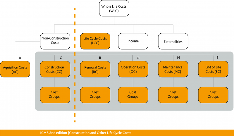
[first figure]
- ‘Occupancy Costs’ are considered part of the ‘Non-Construction Costs’.
- The relationship between Life Cycle Costs and Whole Life Costs as defined by ISO 15686-5:2017 Buildings and constructed assets – Service life planning – Part 5: Life-cycle costing is: as follows:
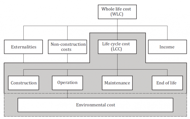
(added, 22/3/2023)
ICMS 3 Definitions in Relation to Life Cycle Costs
- ICMS 3 deals with Life Cycle Costs only, and have defined the following terms (definitions in italics):
- Generally:
- Constructed Asset (or Asset): The output from any building or civil engineering project.
- Life Cycle Costs (LCC):
- Life Cycle Cost: Cost of a Constructed Asset or its parts throughout its life cycle from construction through use, operation, maintenance and renewal till the end of life or a shorter Period of Analysis, while fulfilling the performance requirements (see the [first figure] above).
- Acquisition Costs: All payments or considerations required to acquire / lease / purchase the land, property or existing Constructed Asset, and all other expenses associated with the acquisition, excluding physical construction. [This is not a LCC as defined by ISO 19686 but has been included as a Category by ICMS 3.]
- Construction Costs: Expenditures incurred as a direct result of construction including labour, materials, plant, equipment, site and head office overheads and profits as well as taxes and levies. They are the total price payable for all permanent and temporary works normally included in construction contracts, including goods or materials supplied by the Client for the Constructor to install.
- Renewal Costs: The costs of replacing a Constructed Asset and/or major components once they reach the end of their life, and which the Client decides are to be included in the capital rather than the revenue budget.
- Operation Costs: Costs incurred in running and managing a Constructed Asset during occupation, including administrative support services, rent, insurances, energy and other environmental/regulatory inspection costs, taxes and charges.
- Maintenance Cost: The total cost of labour, material and other related costs to retain a Constructed Asset or its parts so that it can perform its required functions (ISO 15686-5). Maintenance includes conducting corrective, responsive and preventative maintenance on a Constructed Asset or its parts and all associated management, cleaning, services, repainting, repairing or replacing of parts as needed for the Constructed Asset to be used for its intended purpose. It does not include Renewal Costs.
- End of Life Costs: The net costs or fees for disposing of an asset at the end of its service life after deducting the salvage value and other income due to disposal, including costs resulting from disposal inspection, decommissioning and decontamination, demolition and reclamation, reinstatement, asset transfer obligations, recycling, recovery, disposal of components and materials, and transport and regulatory costs.
- Whole Life Costs but not Life Cycle Costs:
- Non-Construction Costs: Includes finance costs, service charges, parking charges and charges for associated facilities.
- Occupancy Costs: Costs that arise exclusively as a result of the occupation of a Constructed Asset, including reception, library services and porterage. Occupancy Costs are part of the Non-Construction Costs.
- Income: Money received from sales and other activities during the life of an Asset. [Not exactly a cost.]
- External Costs: Costs associated with an asset that are not reflected in the transaction costs between provider and consumer, collectively referred to as Externalities. These costs may include business staffing, productivity, social impact costs and user costs and can be considered in a Life Cycle Cost analysis when explicitly identified (ISO 15686-5).
- Externalities: Quantifiable cost or benefit that occurs when the actions of organisations and individuals have an effect on people other than themselves, e.g., non-construction costs, income and wider social and business costs (ISO 15686-5).
- ICMS 3 has defined the following terms (definitions in italics) to deal with time value of money:
- Dates and Periods:
- Reporting Date: The date at which the report describing construction or Life Cycle Costs is compiled.
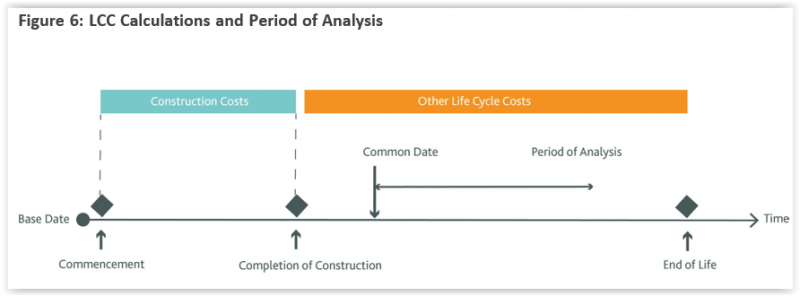
- Common Date: The date to be used in conjunction with Life Cycle Costing, being a date not earlier than the completion of construction. All future cash flows occurring at different times are discounted or compounded as if the costs are incurred at that date. [Unlike ISO 15686-5 which uses “Base Date”, ICMS 3 uses “Common Date” because “Base Date” is generally used in construction contracts as the base date for contract price fluctuations adjustment.]
- Base Date: The date at which the individual Construction Costs in ICMS cost reports apply exclusive of Price Level Adjustments after that date. However, there can be a separate allowance for Price Level Adjustments under the Risk Allowances Group. A different date (the Common Date) applies to Life Cycle Costs.
- Period of Analysis: Period of time over which Life Cycle Costs are analysed as determined by the Client. It may cover the entire life (physical, technical, economic, functional, social, or legal life) or a selected stage or stages or periods of interest as required by the Client.
- Costs and values:
- Present Day Value: Monies accruing in the future which have been discounted to account for the fact that they are worth less at the time of calculation (ISO 15686-5).
- Net Present Value or Cost: The sum of the discounted future cash flows (ISO 15686-5).
- Nominal Cost: The expected price that will be paid when a cost is due to be paid, including estimated changes in price due to, for example, forecast change in efficiency, inflation or deflation and technology (ISO 15686-5).
- Real Cost: The cost expressed as a value at the Common Date, including estimated changes in price due to forecast changes in efficiency and technology, but excluding general price inflation or deflation (ISO 15686-5).
- Inflation/Deflation: Sustained increase/decrease in the general price level of resources (ISO 15686-5).
- Escalation: A positive or negative factor or rate reflecting an estimate of differential increase/decrease in the general price level for a particular commodity, or group of commodities, or resources (ISO 15686-5).
- Discounted Cost: The resulting cost when the real cost is discounted by the real discount rate or when the nominal cost is discounted by the nominal discount rate (ISO 15686-5).
- Rates:
- Discount Rate: Factor or rate reflecting the time value of money that is used to convert cash flows occurring at different times (ISO 15686-5).
- Nominal Discount Rate: The factor or rate used to relate present and future money values in comparable terms, taking into account the general inflation/deflation rate.
- Real Discount Rate: The factor or rate used to relate present and future money values in comparable terms, not taking account of general or specific inflation in the cost of a particular asset (ISO 15686-5).
- Dates and Periods:
- Generally:
(added, 22/3/2023)
Life Cycle Cost Considerations Given by ICMS 3 (cited in italics)
- Setting the scope of the Life Cycle Costs:
- Life Cycle Costing (LCC) is an economic evaluation method that takes account of all relevant costs over a time horizon (Period of Analysis). Presentation of life cycle costs should make clear the scope of those costs included or excluded (as defined in the Categories and Group tables) and the relevant level of costs for the LCC purpose, as well as dealing with the time value of money.
- LCC may be reported at a lesser level of detail than the underlying analysis. For example, the detailed cost analysis may be at Level 4 Sub-Groups, whereas reporting may be at Level 1 Project or Sub-Project or Level 2 Categories or Level 3 Groups.
- LCC may be part of a wider economic project evaluation that considers the Whole Life Costs (including non-construction costs such as finance, business income from sales and disposals, occupancy costs and externalities).
- Expected asset life:
- The design life of the Constructed Asset is a key performance requirement and should be defined in the project brief. The estimated expected service life of the Constructed Asset should be at least as long as the design life.
- Renewals of Constructed Assets during the expected service life should be included in the life cycle cost’s Period of Analysis, as well as any associated end of life or hand-back obligations.
- Time value of money:
- The initial Construction Costs reported should be the forecast or actual final costs to complete the construction of the Project. Forecast costs should include an adjustment for price level fluctuations until the completion of the Project using published market indices and an agreed Base Date.
- The rest of the LCC should be the forecast costs after the completion of construction until the end of life or a shorter Period of Analysis (e.g. one to ten years). This should be defined in the project scope, discounted to a Common Date not earlier than the completion of construction, using Discount Rates mandated by government authorities for public projects or published Discount Rates for the market where the Project is located for private projects or other rates such as those designated by the Client.
- These interrelated terms of LCC are illustrated in Figure 6:
- ICMS can be used to report and compare actual costs which have been collected, recorded and analysed. Actual costs should be recorded in the amounts paid. When historic actual costs are used for forecasting future costs, Price Level Adjustments should be made to bring the historic costs to the desired date of payment. LCC has certain cost variables. It is therefore important to record the purpose, scope, form and method of the economic appraisal as well as the Common Date and the underlying assumptions, risks and uncertainty, information and data sources.
- Net Present Value Calculations
- For option appraisal based on LCC the Net Present Values (NPV) of different options should be compared. The NPV of an option should be a single figure that sums up the present values of all relevant future LCC occurring during the Period of Analysis. NPV is the normal measure for discounted LCC.
- To convert a future cost to the present value (cost) at the Common Date, the following formulae, using $ as an example currency, can be used:
- Present value = future cost × discounting factor
- R% = Discount Rate per annum
(added, 22/3/2023)